Generating training data using general-purpose GNN force field M3GNet and learning neural network force field#

The nanomaterial integrated GUI Advance/NanoLabo has a function to generate training data that can be used in the neural network molecular dynamics system Advance/NeuralMD from the trajectory of molecular dynamics calculations using LAMMPS. Using this function, it is possible to generate training data in a significantly shorter time compared to training data generation using DFT.

In this analysis example, we will generate training data for Si and SiC through molecular dynamics calculations using the general-purpose graph neural network (GNN) force field M3GNet, and use them to learn the Neural Network (NN) force field. The NN force field learned in this way can perform calculations faster than M3GNet while maintaining the same level of accuracy as M3GNet for any system used to generate training data. In addition, in this analysis example, in order to evaluate and compare the performance of force fields, we will also calculate the Young's modulus of Si and SiC using each force field.

Generation of training data using M3GNet#

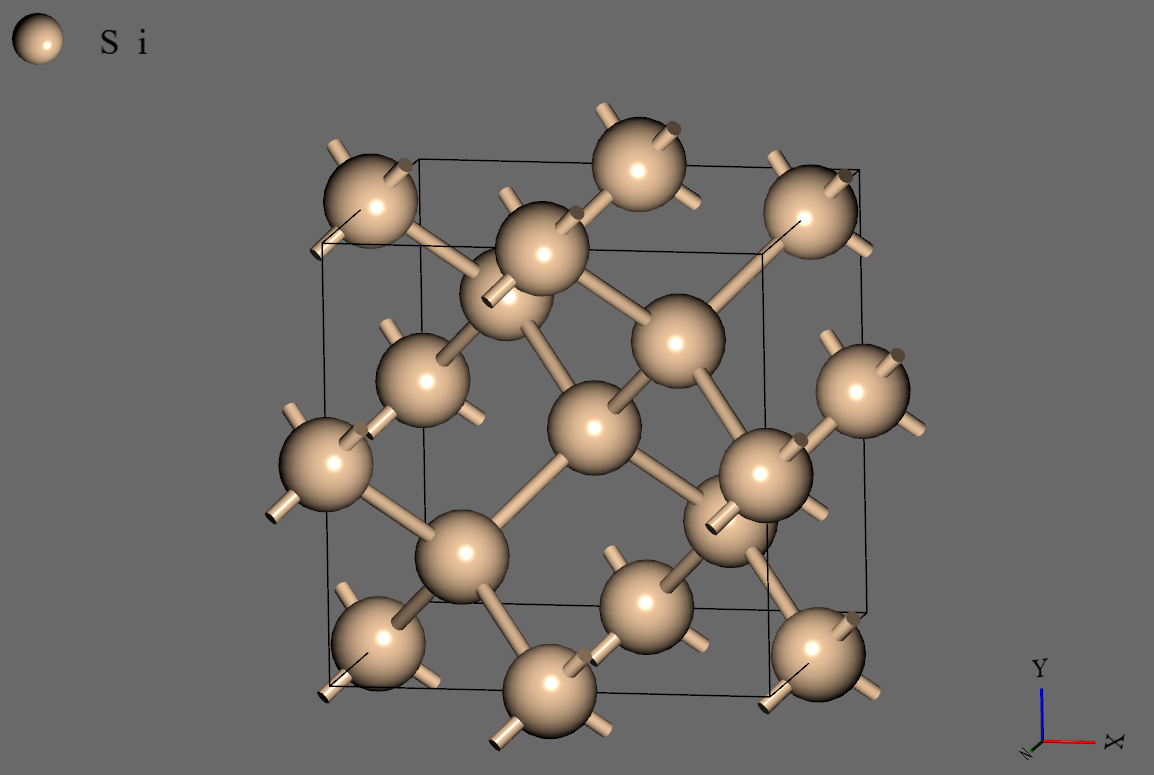
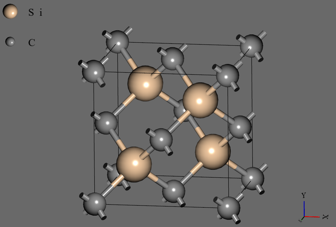
Molecular dynamics calculations using M3GNet were performed for each of the diamond Si unit cell model (mp-149) and 3C-SiC unit cell model (mp-8062) obtained from the Materials Project¹, and training data was generated.

Under the NPT ensemble, the temperature was kept constant at 300 K, the pressure was kept constant at 1 bar, and Triclinic was chosen as the cell deformation constraint. The time step size was 0.5 fs, and the number of steps was 500000 steps (250 ps).

Settings for generating training data can be completed by simply entering dump nnpdump all nnp 100 sannp.train in the User's Additional Settings into Input-file field on the User's screen. When entered like this, information on all atoms will be written to the training data file sannp.train every 100 steps, but the number of steps, target atoms, and file name can be changed as necessary.

We performed calculations under the above conditions and generated 5001 pieces of training data for each of Si and SiC.

Molecular dynamics calculations for Si and SiC were completed in 1 hour 10 minutes and 1 hour 28 minutes², respectively, indicating that training data can be generated in a significantly shorter time than when using DFT calculations.


Si model	SiC model

Neural Network Learning#

For each of Si and SiC, we trained the NN force field using the training data generated in the previous section.

The learning conditions were set as follows.

Δ-NNP method: ON (LJ-like Potential)
Symmetric function: Chebyshev polynomial (50 radial components, 30 angular components)
Cutoff function: tanh(1-r/r0)^3 (cutoff radius 6 Å)
Neural Network structure: 2 layers x 40 nodes x 16 model ³
Activation function: twisted tanh
Number of epochs per Super Epoch³: 500
Number of training data per Super Epoch: 500
Energy convergence threshold: 0.001 eV/atom
Force convergence threshold: 0.01 eV/Å

Furthermore, 10% of the training data was separated as test data, and the remaining 90% was used for learning.

The following table shows the RMSE of the NN force field obtained as a result of training and testing.

	Energy RMSE(learning) (eV/atom)	Energy RMSE(test) (eV/atom)	Force RMSE(learning) (eV/Å)	Force RMSE(test) (eV/Å)
Si	4.905×10^-3	5.175×10^-3	4.792×10^-2	5.040×10^-2
SiC	3.058×10^-2	2.681×10^-2	1.320×10^-1	1.646×10^-1

In addition, both Si NN force field learning⁴ and SiC NN force field learning⁵ 5 were completed in about 10 minutes.

Young's modulus calculation#

Using M3GNet and the NN force field generated in the previous section, we performed molecular dynamics calculations for the 2×2×2 supercell models of Si and SiC, and calculated the Young's modulus from the results.

In this example, we calculated the change in stress when the cell was deformed at a constant speed in the same way as the previous Calculation of anisotropic Young's modulus of single-crystal Ni via molecular dynamics simulation. However, the number of steps for the equilibration scheme was 5000 steps (5 ps), the uniaxial stress scheme was 500000 steps (500 ps), and the rate of cell deformation was 2 × 10^-4Å/ps in the <100> direction.

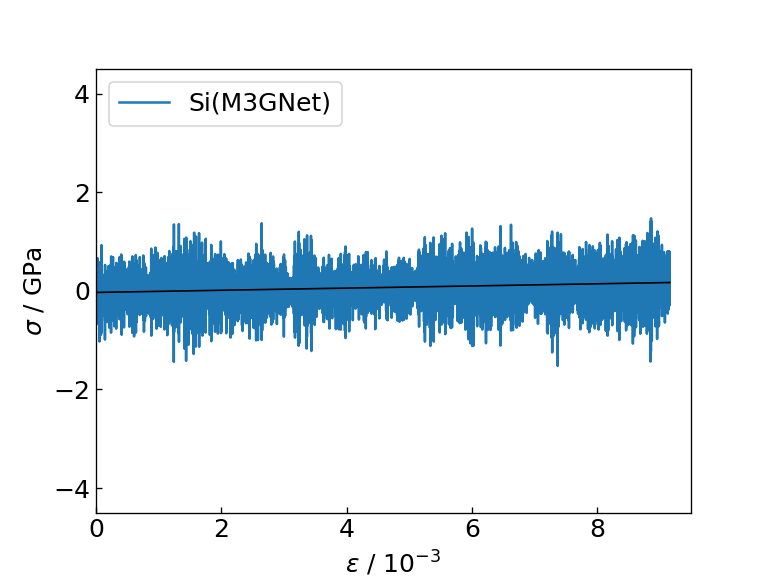
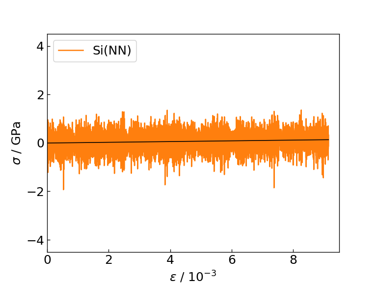
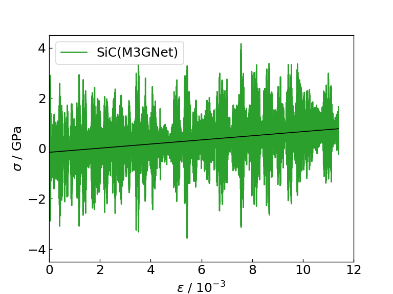
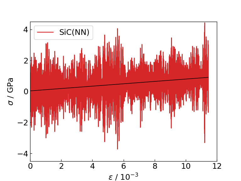
The graph and table below show the graph of the stress $\sigma$ response to strain $\epsilon$ obtained as a result of the calculation, the Young's modulus obtained as the slope of the linear function fitting (black solid line), and the time required for each calculation. For comparison, the table also shows literature values for the Young's modulus of Si and SiC determined by DFT calculation.


Strain-stress diagram of Si (M3GNet)	Strain-stress diagram of Si (NN)

Strain-stress diagram of SiC (M3GNet)	Strain-stress diagram of SiC (NN)

	Young's modulus by M3GNet (GPa)	Young's modulus by NN force field (GPa)	Young's modulus by DFT (GPa)
Si	22	15	138.5⁶
SiC	82	76	362⁷

	Computation time by M3GNet	Computation time using NN force field
Si	3 hours 57 minutes ²	25minutes ⁴
SiC	7 hours 51 minutes ²	55minutes ⁵

From the figures and tables, it can be seen that the NN force field calculates the force response and Young's modulus to strain with the same accuracy as M3GNet. On the contrary, when using the NN force field, calculations can be executed approximately 8 times faster than M3GNet, indicating that the NN force field can be applied to calculations for larger systems compared to M3GNet.

Note that the Young's modulus calculated by M3GNet and the NN force field is estimated to be smaller than the Young's modulus calculated by DFT calculation, but this is due to the trained model of M3GNet that is distributed as MP-2021.2.8 This is thought to be due to the calculation accuracy of Young's modulus of Si and SiC (EFS). On the other hand, the table shows that the relationship between the Young's modulus of Si and SiC can be calculated qualitatively correctly in both cases of M3GNet and NN force field.

From the above results, by using Advance/NanoLabo and Advance/NeuralMD, we can create a NN force field that can perform calculations in a significantly shorter time while maintaining the same accuracy as a general-purpose force field for a specific system. I found out that it can be generated. By using this function, it is expected that calculations on large-scale systems that could not be calculated using general-purpose force fields can be performed in a relatively short time.

Generating training data using general-purpose GNN force field M3GNet and learning neural network force field#

Generation of training data using M3GNet#

Neural Network Learning#

Young's modulus calculation#

関連ページ#