Benchmarking of training data creation, neural network training, and molecular dynamics simulation#
To run a neural network molecular dynamics simulation using Advance/NeuralMD, following 3 steps:
- Creating training data (Quantum ESPRESSO)
- Training a neural network (Advance/NeuralMD)
- Molecular dynamics simulation (LAMMPS)
are required. Since all of these calculations are quite heavy when dealing with practical systems, they should be performed using a workstation with many CPU cores or a machine called a cluster.
In this article, a machine with specifications similar to those used in actual calculations is prepared and the results of each of the three steps of the calculation are shown. Please use this as a reference to estimate the calculation time.
Computing environment#
- CPU: 3rd generation (Ice Lake) Xeon 24-core 2.6GHz x 2 (48 cores total)
- Memory: 32GB DDR4-3200 ECC RDIMM x 16 (512GB total)
- OS: AlmaLinux 8.3
HPC Systems cooperated in the preparation and use of the computing environment.
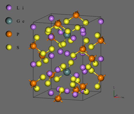
Target System#
Calculations were performed on Li10GeP2S12 (LGPS). This material is expected to be used as a solid electrolyte in all-solid-state lithium ion batteries.
Benchmark 1: Training Data Creation#
First-principles electronic structure calculations were performed using Quantum ESPRESSO 6.7 (Advance Software modified version, included with Advance/NanoLabo Tool). Executing the calculations for each with a number of different atomic structures as input, training data was obtained as an output file.
Quantum ESPRESSO was executed with MPI parallels. In this case, one method is to perform parallel calculations using all the cores in the computer (48 parallel cores in this case) one by one, however, too many parallel cores may reduce efficiency, or the calculation may fail in the first place. Therefore, a pattern with reduced number of parallels and instead with simultaneous multiple calculations (e.g., two 24-parallel calculations were executed in parallel) was also tried.
In this environment, OpenPBS 20.0.1 was installed, and each calculation was submitted and executed as a job.
To check for the case with different number of atoms, the original structure (50 atoms) and a 2 x 2 x 1 supercell (200 atoms) were prepared, and following two ways were tried.
- 50 atoms x 500 structures
- 200 atoms × 125 structures
Since training data was obtained for each atom, the number of data was the same for both.


The plot of the resulting walltime, where cputime_sum is the sum of the runtimes for each job and walltime_max is the runtime for the longest job, the latter being the actual time to take for calculations.
- Efficiency was high at MPI parallel numbers of 12 to 16, and parallelization efficiency declined at higher numbers and walltime increased.
- Conversely, even if the number of MPI parallels for each job was small, the walltime became longer as more jobs were executed simultaneously. It seems that there was a bottleneck associated with the simultaneous execution of many jobs, such as file access.
- There was also a difference depending on with or without MPI parallel, and walltime was shorter when the MPI parallel number was 1 (parallel computation is not used). In particular, the case of 200 atoms had the shortest walltime even though 48 jobs were executed simultaneously.
Benchmark 2: Neural Network Training#
Neural network training using Advance/NeuralMD 1.4 was performed. The combined training data from the previous section (50 atoms x 500 structures + 200 atoms x 125 structures = 50000 atoms) was used.
This time, only one calculation was performed. Using hybrid of MPI and OpenMP parallels, multiple patterns were tested under the condition that the number of MPI parallels x the number of OpenMP parallels = the number of all cores (48). The number of epochs was fixed at 10000.

The plot of the resulting walltime.
- MPI parallel was more efficient than OpenMP parallel, with the largest MPI parallel numbers of 48 having the shortest walltime.
Benchmark 3: Molecular Dynamics Simulation#
A molecular dynamics simulation using LAMMPS 7Aug2019 (Advance Software modified version, included in Advance/NanoLabo Tool) was performed. The neural network force field trained in the previous section was used.
In this calculation, also using a hybrid of MPI and OpenMP parallels, multiple patterns were tested under the condition that the number of MPI parallels x the number of OpenMP parallels = the total number of cores (48).
Using LGPS supercell (1200 atoms), the NVT calculations at 300 K for 2000000 steps (1 ns) were performed.

The plot of the resulting walltime.
- Hybrid of about 12 MPI parallels x 4 OpenMP parallels was more efficient.
Summary#
Based on the above results, the estimated walltime for each process is shown below. For training data creation, the number of structures was 5000 that had been multiplied by a factor of 10 to make the value more practical.
| Process | Calculation time | Content | Parallels |
|---|---|---|---|
| Training data creation | 6.3 hours | 5000 structures | MPI16-parallel×3-job simultaneous executed in parallel |
| Neural Network training | 11 mintues | 50000 atoms | MPI48-parallel |
| Molecular Dynamics calculation | 19.5 hours | 2000000 steps(1 ns) | MPI12×OpenMP4-parallel |
In this computing environment, it turned out that a set of calculations could be done in about one to two days.
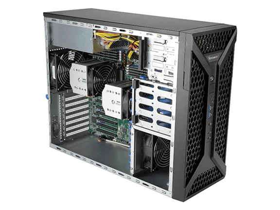
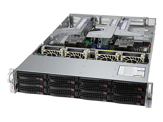
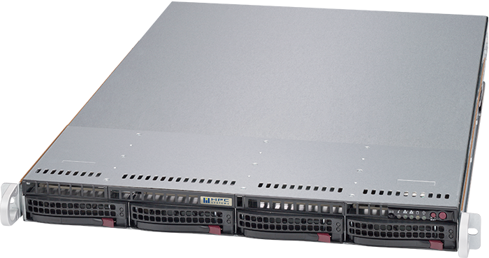
Reference: Specific examples of machines used for calculations#
HPC Systems has listed several machines that can be used for Advance/NeuralMD calculations.
Workstation#
Rackmount#
Of course, other machines with various configurations are available according to budget and required specifications. If you are considering purchasing a machine, please contact HPC Systems.