Conductivity Calculation of Lithium Ion Conductor LGPS by Δ-NNP Method#
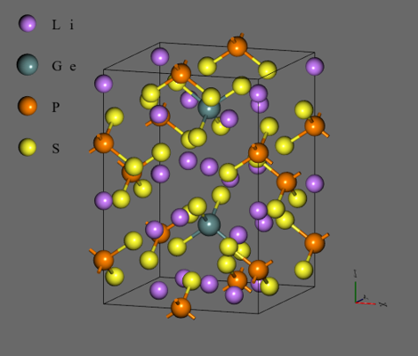
Li10GeP2S12#
- Li10GeP2S12 (LGPS)is a lithium ion conductor with high ionic conductivity of more than 10-2 S/cm at room temperature and is expected to be used as a solid electrolyte in all-solid-state lithium ion batteries.
- The tetragonal unit cell contains two [GeS4]4- of tetrahedral structure, four [PS4]3-, and 20 Li+.
- The ionic conductivity was calculated for these crystals by applying the Δ-NNP method, a new Neural Network force field method originally developed by us.
Δ-NNP Method#
- In the usual Neural Network force field (NNP) method, the total energy 𝐸tot of the system is expressed in terms of the energy 𝐸NNP calculated by NNP: 𝐸tot=𝐸NNP
- We have uniquely developed a differential NNP method (Δ-NNP method), which is an improvement of the NNP method, and implemented it in our own product, NeuralMD. Δ-NNP method expresses the total energy 𝐸tot as the sum of the energy 𝐸C calculated by the classical force field and the energy 𝐸NNP calculated by NNP: 𝐸tot=𝐸C+𝐸NNP
- For the classical force field, Lennard-Jones-like two-body potential is used:
- The training data for Neural Network is not the energy calculated with DFT itself, but the difference between the energy with DFT and with classical force field .
- In inorganic crystals, it is known that Lennard-Jones and Buckingham two-body functions can represent most of the structure of potential topography. We have adopted the approach of applying two-body functions as the zeroth approximation of the potential topography, and supplementing the excess portion that cannot be fully expressed by two-body functions with NNP method. As a result, NNP expresses the topography with only less unevenness and can handle the crystalline system without fully demonstrating true values of a Neural Network. In other words, a Neural Network has enough power left over in the normal state of crystalline systems. On the other hand, in special situations, such as when defects, impurities, surfaces, interfaces, and ions are in intense motion, this extra power of a Neural Network comes into play.
- The application of Δ-NNP method has been successful in (1) improving convergence of a Neural Network learning process and (2) creating a useful force field even with a small amount of training data.
Initial Force Field Creation#
- First, an initial force field was created with a small number of training data. Then, the number of training data was increased by reinforcement learning.
- The unit cell of Li10GeP2S12 (50-atom system) was used as training data for an initial force field. The crystal structure obtained from Materials Project (mp-696128) was used as it was. The atomic coordinates were randomly displaced by 0.1~0.2 Å to generate a large number of structures, and SCF calculations were performed on each structure, whose results were used as training data. The number of structures employed in the training data was 714. Quantum ESPRESSO was used for SCF calculations, with ultrasoft pseudopotentials, the cutoff energy of 40 Ry, and k-point sampling of only Γ points.
- Force fields were optimized using the generated training data. First the two-body force field were optimized and then the Neural Network was trained. For comparison, a regular HDNNP without the two-body force field was also created. Both of Δ-NNP and HDNNP have RMSE(Energy) 1.4meV/atom and RMSE(Force) 0.08eV/Å converged.
- 80 Chebyshev functions were used for the symmetry functions in NNP. The cutoff radius was 6 Å. The structure of the Neural Network was 2 layers x 40 nodes and the activation function was twisted tanh.
MD Trial Calculation Using an Initial Force Field#
- MD calculations were performed using the created initial force field, for an NVT ensemble with T=800K, Δt = 0.5fs, and a simulation time of 100 ps.
Calculation Results of Δ-NNP
Structure at t = 100 ps
.png)
Radial Distribution Function
.png)
- The tetrahedral structure of [GeS4]4- and [PS4]3- was preserved.
- Stability to withstand high temperatures of 800 K were realized with only about 700 training data, which were just randomly displaced atoms!
- The scheme of generating an initial force field with a small amount of training data → adding structures by MD and MC in the initial force field → implementing reinforcement learning can be easily realized.
Calculation Results of HDNNP
Structure at t = 100 ps
.png)
Radial Distribution Function
.png)
- HDNNP could not withstand temperatures as high as 800K, and its structure would fail completely. This was because extrapolation did not work.
- Reinforcement learning using trajectories cannot be implemented.
Reinforcement Learning#
- Metropolis method was performed using an initial force field to generate a large number of new structures, with temperatures ranging from 300 K to 1000 K. The number of structures in the final training data was 6,914. 200 structures of those are 2 x 2 x 1 supercells while all other structures were unit cells. 10,000 epochs learning in L-BFGS method was performed.
- RMSE(Energy) = 3.4 meV/atom , RMSE(Force) = 0.077 eV/Å
- Δ-NNP showed better convergence than HDNNP (figures below).
.png)
.png)
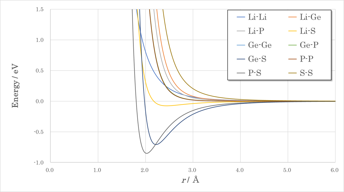
Two-body Potential Function#
- Accuracy when using only two-body potentials (without NNP):
RMSE(Energy) = 41.9 meV/atom , RMSE(Force) = 0.457 eV/Å
- Ge-S, P-S, and other bonds were correctly represented (a figure below).
Calculation of Diffusion Coefficient of Li Ion#
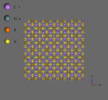
- Using a 1600 atom supercell model (right figure), MD calculations from 0.5 to 1.0 ns were performed. Δt = 0.5 fs, NVT ensemble.
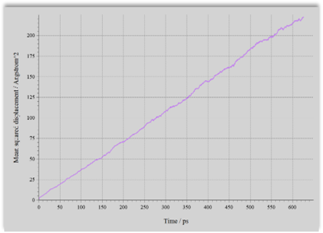
- Simulations were performed for various values of temperature from 350 to 800 K. The diffusion coefficient of lithium ions was evaluated from the slope of the MSD.
- In general, at high temperatures, motions of atoms are large and diffusion coefficient can be evaluated with high accuracy even with a small model size. Conversely, at low temperatures, accuracy of diffusion coefficient cannot be guaranteed unless the model size is sufficiently large. Therefore, although diffusion coefficients can be calculated even with first-principles MD at high temperatures, the NNP method is required at low temperatures.
LGPS Super Cell Model
MSD of Li Ion
Ion Conductivity#
- If the diffusion coefficient is 𝐷, the ionic conductivity 𝜎 of Li+ is given by the following equation: 𝜌 is the concentration of Li+, 𝑒 is the elementary charge, 𝑘 is Boltzmann's constant, 𝑇 is the temperature.
- Arrhenius plot of the calculated 𝜎:
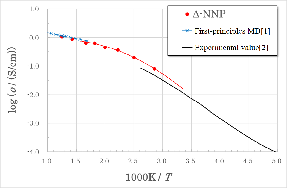
- [1] A.Marcolongo, ea al., https://arxiv.org/abs/1910.10090
- [2] Ryoji Kanno, Electrochemistry, 85(9), 591–596 (2017)
- The ionic conductivity at T = 298.15K was predicted by interpolating with a quadratic function
σ = 1.6 x 10⁻² S/cm
which is quite close to the experimental value of 1.2 x 10⁻² S/cm. - Since ionic conductivity can be predicted more accurately with a lower cost than first-principles MD or existing NNPs, it is expected to be applied to solid electrolytes other than LGPS.
- It took less than one week from preparation of training data to calculation of σ.