A Neural Network Force-Field Molecular Dynamics Study: Analysis of Iron degradation by Hydrogen#
In molecular dynamics simulations, a total potential energy from a given atomic structure is obtained based on a function. This function is generally called a "force field", having an empirically determined equation. On the other hand, neural network force fields are built without using empirical knowledge. In this case study, we present an example of molecular dynamics simulation analysis of the degradation of iron by hydrogenation. The EAM (Embedded Atom Method) is known as a suitable force field for metals, but this time, instead of using an existing force field, a neural network force field was developed using Advance/NeuralMD to investigate Young's modulus, which is used as an index to stiffness, from the stress response when iron with hydrogen addition.
Obtaining training data and training of neural network#
In a neural network force field, the "energy of an atom and the force acting on that atom" is calculated for each atom in the system from the "atomic structure in the neighborhood. Therefore, it is necessary to prepare a variety of " atomic structures" that can appear in the actual system as training data which is used for training the neural network.
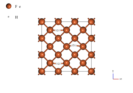
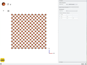
In this case study, a supercell model was used by expanding the body-centered cubic structure unit cell (mp-13)1 from the Materials Project by 3 × 3 × 3. The number of iron atoms is 54, and hydrogenated iron is modeled by adding 3 hydrogen atoms. The model used to develop the force field is shown in the figure below.
Using this model, a neural network force field was developed using the self-learning hybrid Monte Carlo (SLHMC) method. The details of the SLHMC calculation are shown below.
- QE calculations were performed by the NVT ensemble. The temperature was set at 300 K.
- The exchange-correlation functional in the SCF calculations was Pseudopotential, using fe_pbe_v1.5.uspp.F for iron and h_pbe_v1.4.uspp.F for hydrogen. The energy and charge cutoffs were set to 40.0 Ry and 225.0 Ry, respectively.
- The Chebyshev function was used for the symmetry function in NNP. The number of radius and angle functions were set to 50 and 30, respectively. The Neural Network was 40 nodes x 2 layers, and twisted tanh was used as the activation function.
- The initial force field was created by performing 200 steps of First principle molecular dynamics (FPMD). The NNP-MD was performed at 2.5 fs ~ 500.0 fs for each SCF calculation. The training data and NNP-MD were updated every time the number of training data increased by 100. The training data included both accepted and rejected data with 2600 structures.
Simulation model and scheme set up for MD#
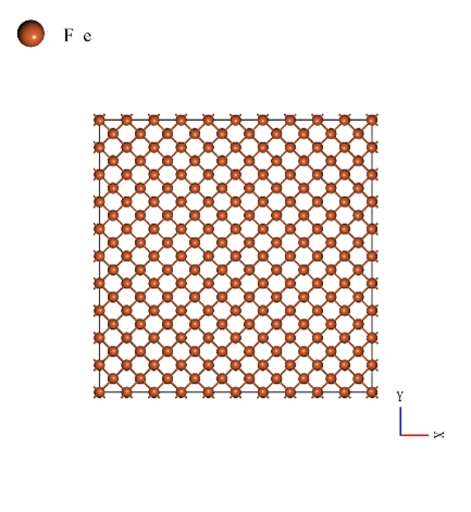
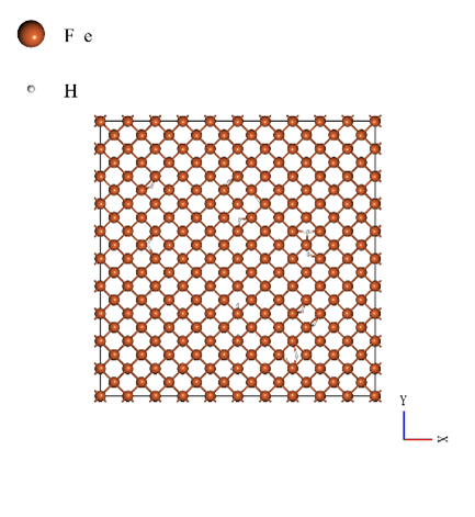
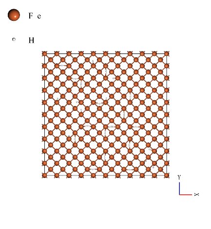
The body-centered cubic structure unit cell (mp-13) which is used in the SLHMC calculation is expanded to 10 x 10 x 10 for the MD simulation. The number of iron atoms is 2000. The iron degradation analysis was performed by comparing Young's modulus of the pure iron and the case with 20, and 40 hydrogen atoms (hydrogen concentration of 1.0% and 2.0%). The models used in the calculations are shown below (from left to right: hydrogen concentrations of 0.0%, 1.0%, and 2.0%).
 |
 |
 |
|---|---|---|
The MD simulation scheme consisted of three steps.
- First, energy stabilization (Optimization) was performed to relax the total energy of the system.
- The system was then equilibrated with 100,000 steps (50 ps) at 300 K and 1 bar. The time step was set to 0.5 fs, and only isotropic deformation was allowed in the cells.
- Next, the virial stress was calculated for each model by applying a strain of 0.001 Å/ps in the x direction for 500,000 steps (500 ps). The time step was set to 1.0 fs. Since the purpose of this simulation is to measure uniaxial stress, the pressure in the direction perpendicular to the direction of strain was set to be constant at 0 bar.
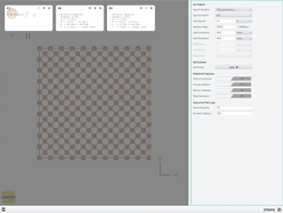
In Advance/NanoLabo, cell deformation in any direction can be easily set from the Option tab. The User's tab allows the definition, calculation, and graphical visualization of physical properties. In this simulation, the user's tab was used to set up the calculation of virial stress. The following are screenshots of the simulation scheme and the Option tab.
 |
 |
|---|---|
Tips The input file can be directly edited before the running the simulations. By editing a line to "fix ensemble, all npt temp 300.0 300.0 0.1 y 0 0 1.0 z 0 0 0 1.0" in the script, the pressure in the y and z directions can be set to remain constant at 0 bar.
MD simulation results#
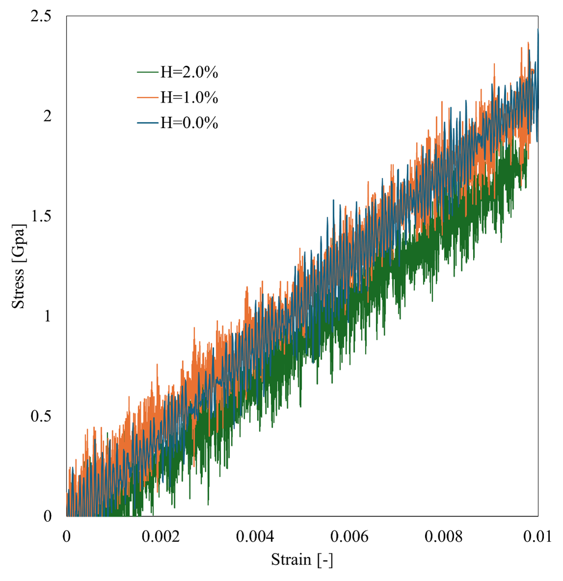
Advance/NanoLabo allows easy visualization of the calculation results on the GUI and output of CSV files. Young's modulus is defined as the ratio of strain to stress. We calculated Young's modulus by fitting the stress-strain curve with a linear regression. The stress-strain curves and the resulting Young's modulus for are shown in the table.
Our results show that Young's modulus of pure iron at 0.0% hydrogen concentration is 218.98 Gpa, which is generally in good agreement with the experimental results in the range of 201-216 Gpa2; thus, this analysis is validated. Young's modulus at 1.0% and 2.0% hydrogen concentration is 208.51 Gpa and 195.42 Gpa, respectively. Compared with the results for pure iron, Young's modulus is reduced by hydrogen addition, which reproduces the iron degradation phenomenon.
This approach can be applied to the degradation phenomena with hydrogen addition for various materials, not only iron.
| Hydrogen concentration (%) | Young's modulus (GPa) Simulation | Young's modulus (GPa) Experiments |
|---|---|---|
| 0.0 | 218.98 | 201-216 |
| 1.0 | 208.51 | - |
| 2.0 | 195.42 | - |