Benchmarking Molecular Densities by Molecular Dynamics Calculations Using a General-Purpose Graph Neural Network (GNN) Force Field#
In this article, I present an example of density calculation that utilizes Advance/NanoLabo, an integrated GUI for nano-materials analysis. In this case study, I used its molecular dynamics functionality (LAMMPS1) to obtain the densities of molecules (water: , benzene: , dichloromethane: ).
Specifically, I placed 10 molecules in the model space and performed molecular dynamics calculations. In molecular dynamics calculations, the force field that describes interatomic interactions is important. Therefore, in this work, I changed the settings of a general-purpose Graph Neural Network (GNN) force field2 and evaluated, as a benchmark, how the differences affect the calculation results. The target systems were water, dichloromethane, and benzene.
Setup of Target for Calculation : H2O#
Here, taking the water molecule as an example, I describe how to configure Advance/NanoLabo. I obtain the molecular structure from the Materials Project3 and set the calculation conditions.
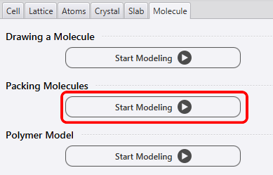
Follow the steps below to build the molecular environment. First, configure the molecule from the Modeler. In the Molecule tab, click “Start Modeling” (red box) of “Packing Molecules” in the figure below to set the molecule packing.
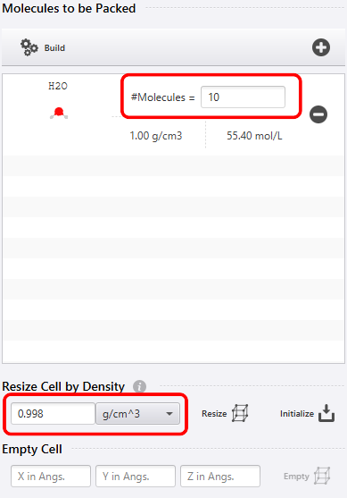
Next, set the Molecules of H2O in the figure below to 10. With this, you can perform a calculation such that 10 water molecules are included in the space. Also, in advance, by using “Resize Cell by Density” to set the density close to the experimental value, I make the steady state of the density reach as quickly as possible. For this reason, I set the density of the water molecule to 0.998.
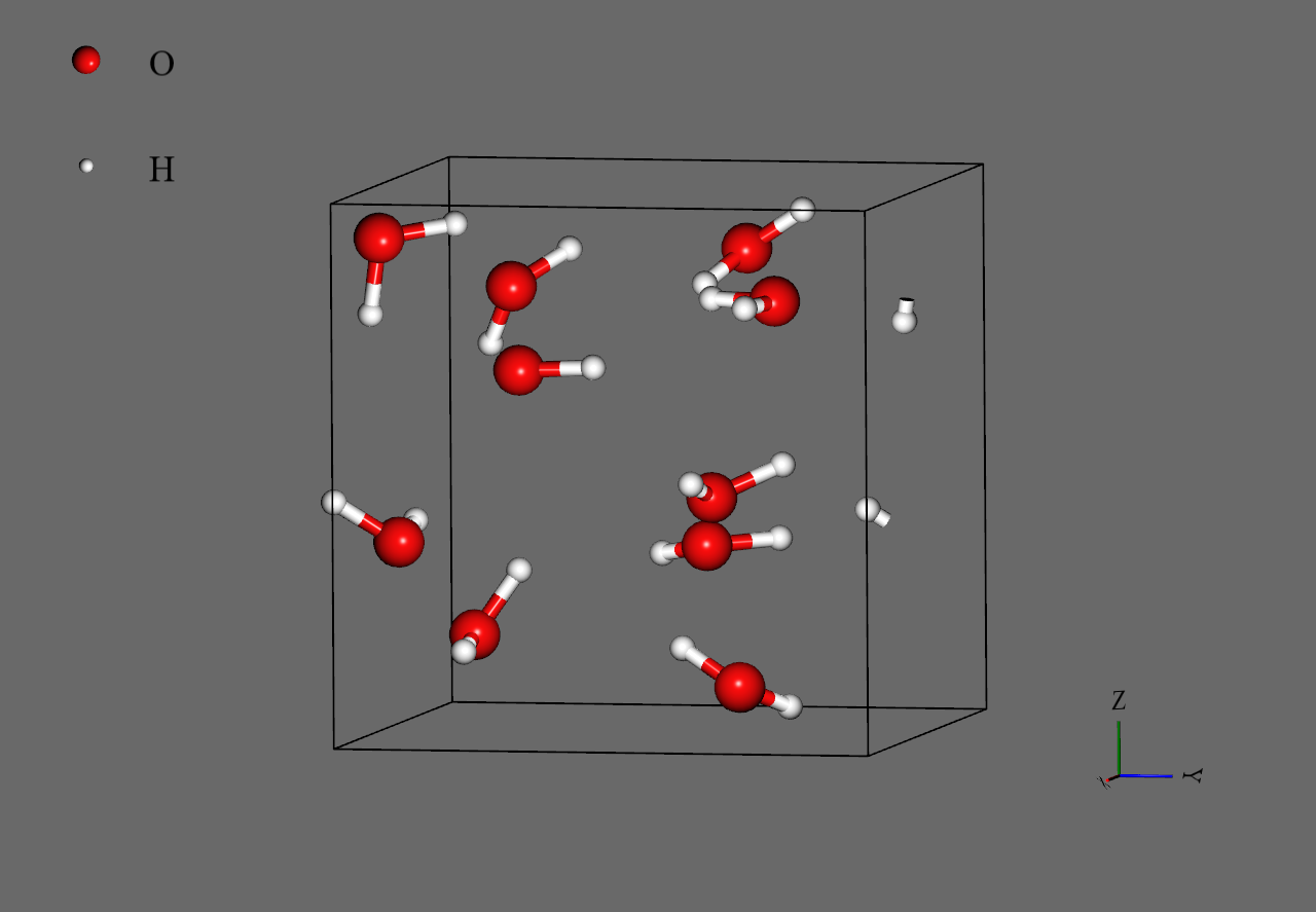
This completes the model settings. Differences may occur in the molecular arrangement, but if it looks like the image below, it has been configured. By time-evolving this configured space, I investigate the change in density.
Analysis Procedure#
Force-Field#
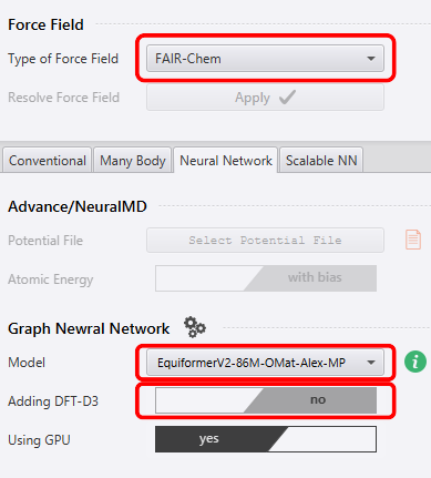
I used LAMMPS as the calculator and compared results by changing three items under Force-Field in the bottom-right menu: - Type of Force Field - Model - Adding DFT-D3
I perform calculations by changing the three red-boxed parts in the image below.
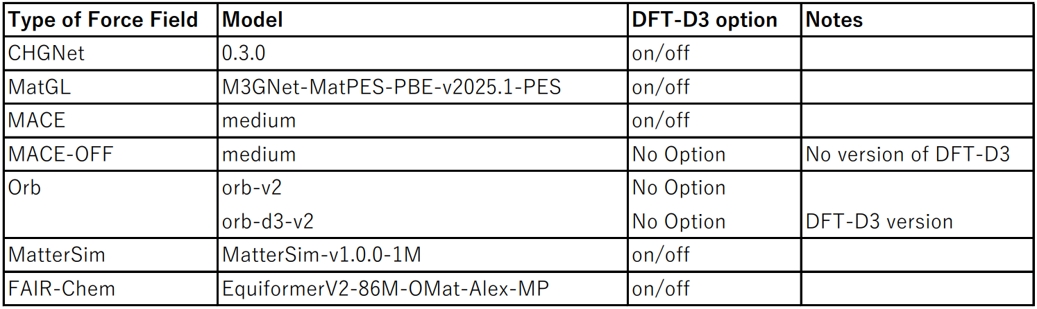
The combinations calculated this time for the three items above are summarized in the table below. For the DFT-D3 option (Adding DFT-D3), there are cases where it is available and cases where it is not; when it was available, I performed calculations both with and without the DFT-D3 correction. In Orb, “orb-d3-v2” corresponds to the case where the DFT-D3 correction is used.
Scheme#
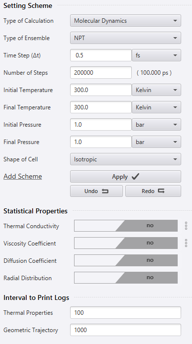
The Scheme settings are shown in the figure below. I performed the molecular dynamics calculation in the NPT ensemble. Because it is the NPT ensemble, the number of particles , pressure , and temperature are constant, and only isotropic deformation of the cell is allowed in the calculation. Here I assume a steady state at 50 ps and take the average of the density of the time steps after 50 ps.
Analysis Results#
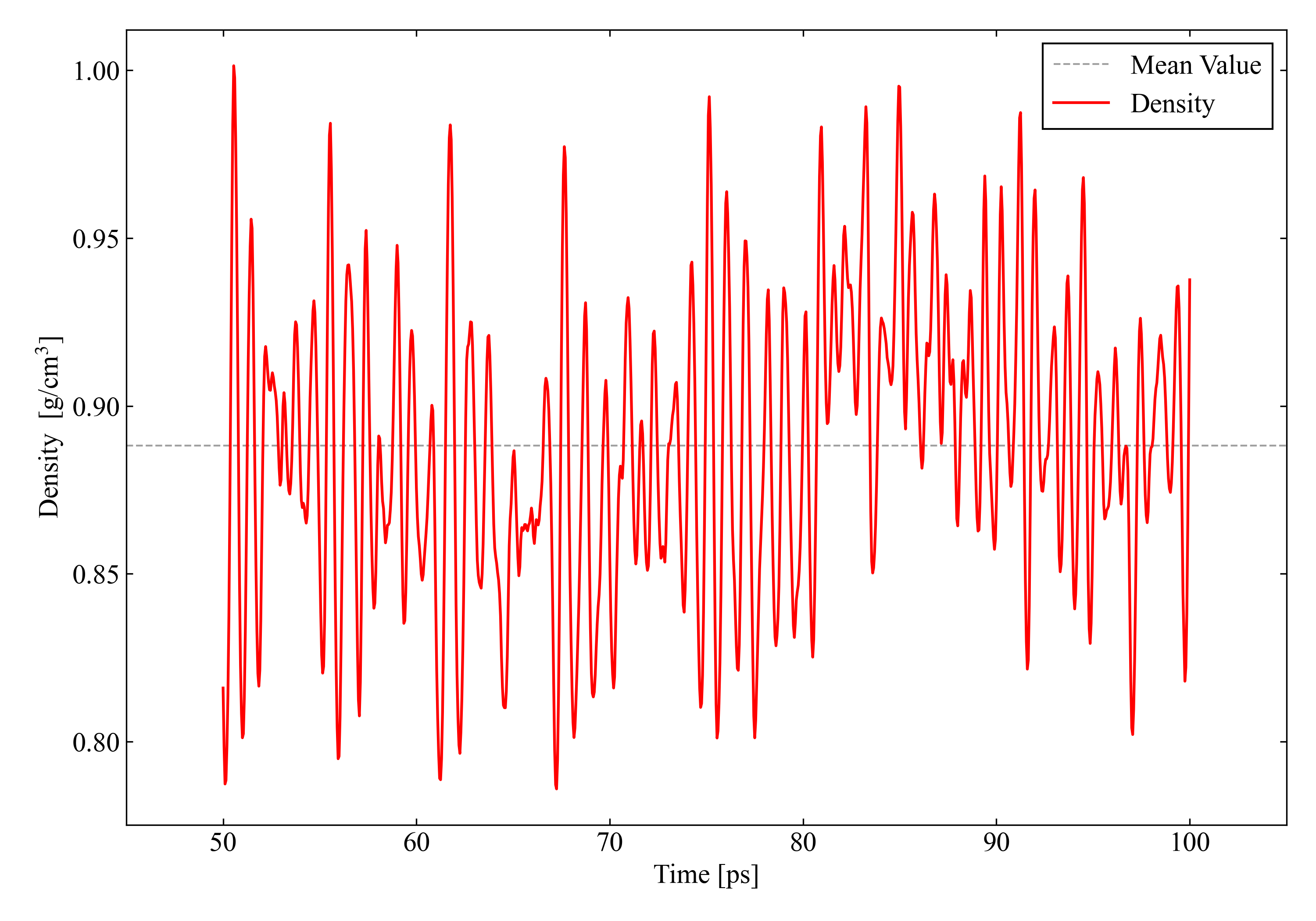
The change in density at steady state when the DFT-D3 correction is not applied to CHGNet is shown in the figure below. The gray dashed line represents the average value. In this case study, for all systems I take as the comparison target the average density over the time steps after 50 ps, and note that I use the value of this gray dashed line as the representative value of each model.
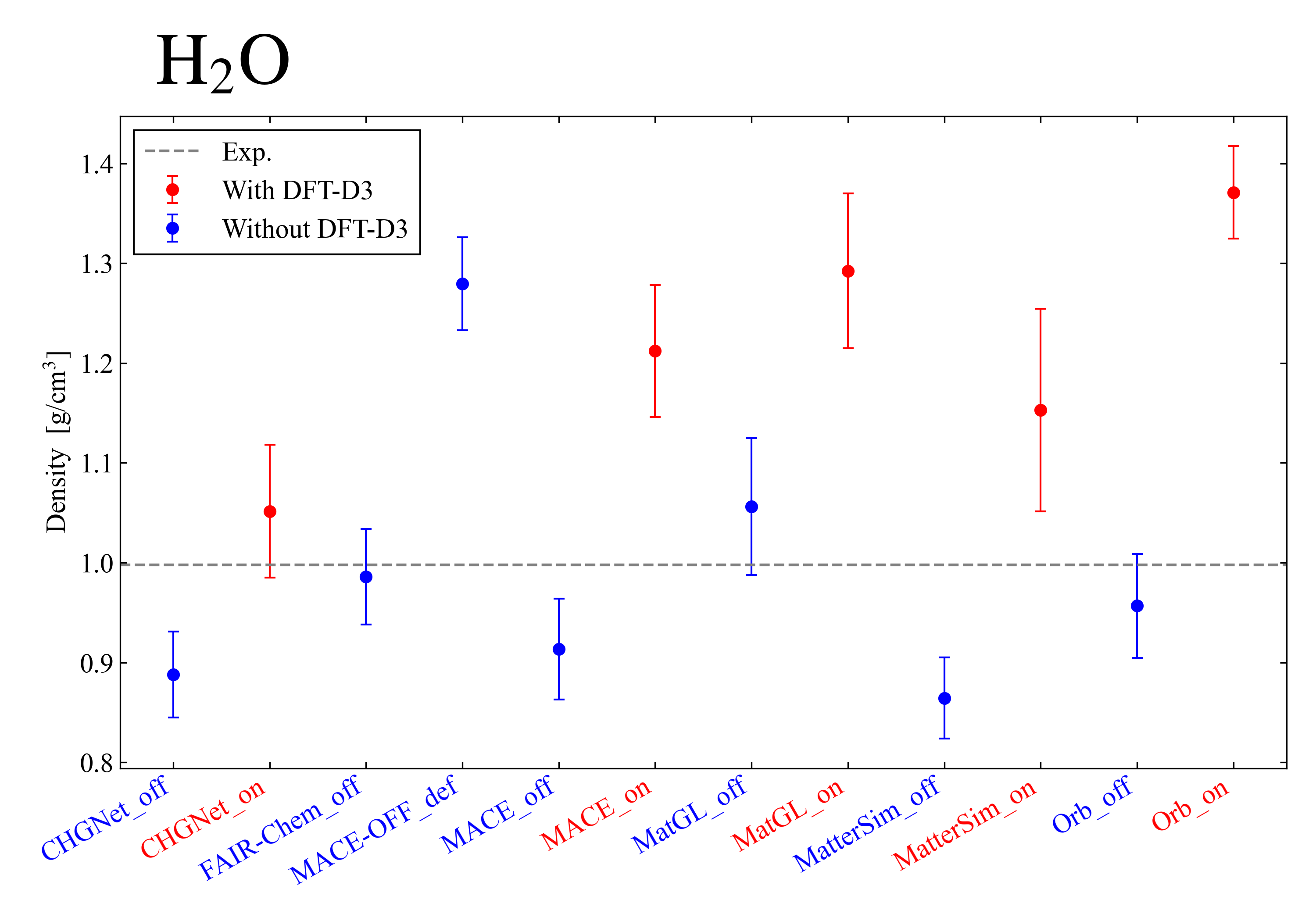
Summarizing the calculation results of the models handled this time, the water molecule became as shown in the figure below. In the systems handled here, not using DFT-D3 yielded results closer to the actual value 0.998. It was also found that using the DFT-D3 correction tends to produce larger error bars. These results are considered to arise because, as the system handled here is small, the attractive effect of the DFT-D3 correction becomes too strong and leads to overestimation. Because the water molecules form hydrogen bonds, it was difficult to reproduce the experimental values.
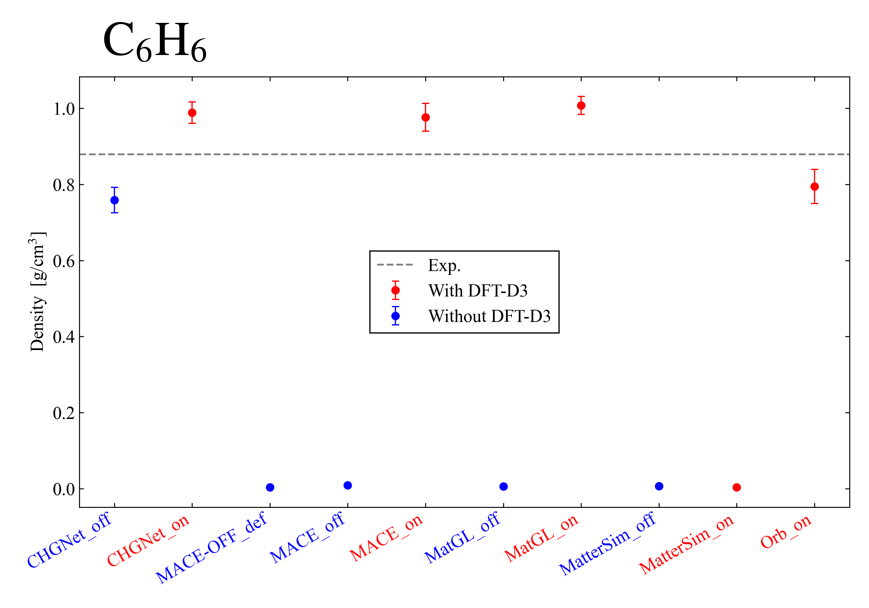
Next, I show the results for benzene: . When it becomes a value close to 0.0, it means that the attraction is too weak and the system diverged. In MatterSim, divergence occurred even when the DFT-D3 correction was applied, which is thought to be due to the smallness of the system. On the other hand, in the other models, it was confirmed that introducing the DFT-D3 correction improves the reproducibility of the experimental value.
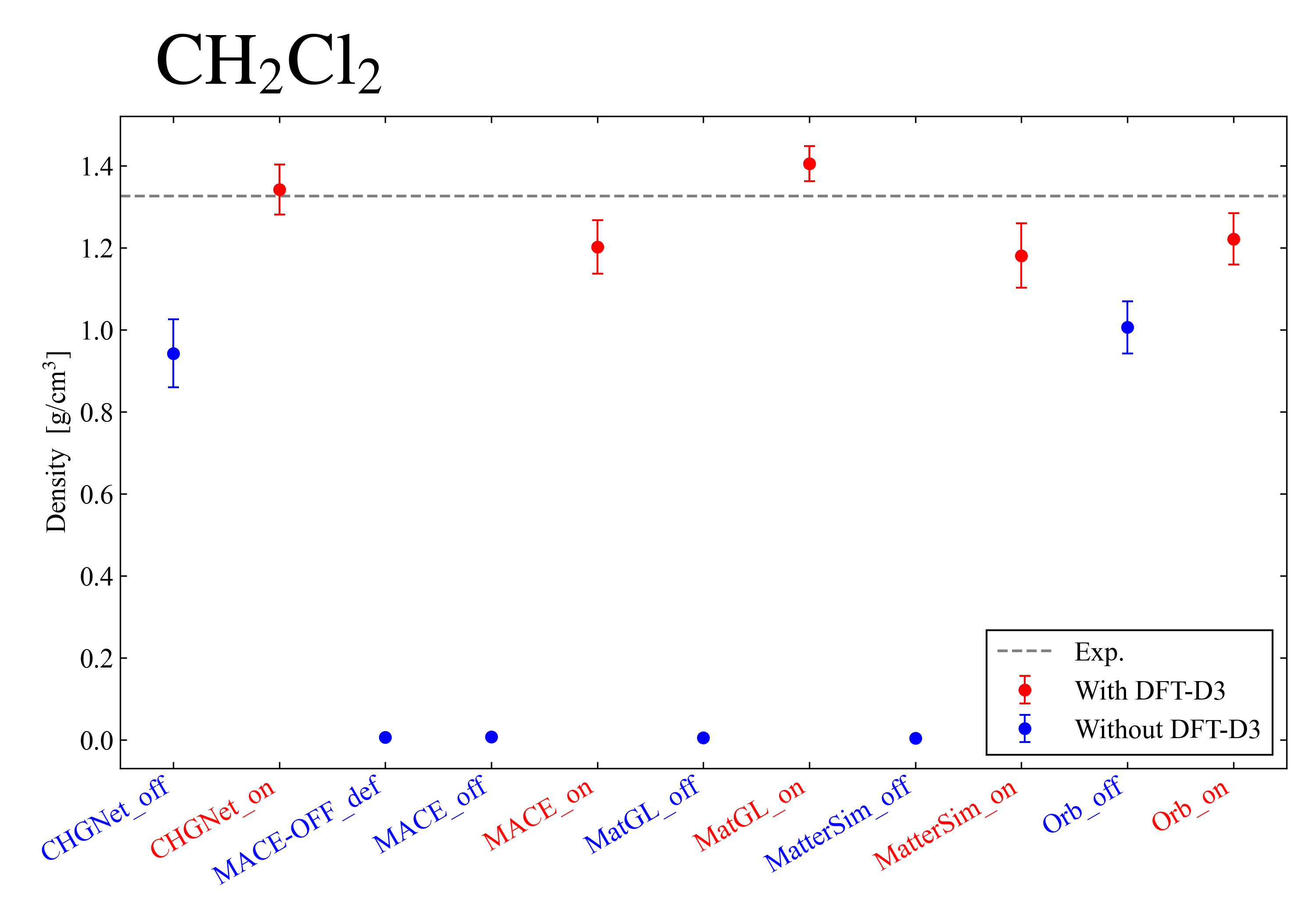
Finally, I show the results for dichloromethane: . By applying the DFT-D3 correction, it was confirmed that in all models the density approaches the experimental value. Also, in all models a tendency was observed for the divergence of the system to be suppressed. From the above, it became clear that, if the system is appropriate, the DFT-D3 correction greatly improves the reproducibility of the experimental value.
Summary#
In this case study, I performed molecular dynamics calculations using the integrated GUI for nano-materials analysis Advance/NanoLabo and evaluated the influence of a general-purpose GNN force field on density calculations. Specifically, I built a model space including 10 molecules each of water, benzene, and dichloromethane, performed simulations under NPT ensemble conditions, and compared the steady values of the density.
As a result of the analysis, while the DFT-D3 correction does not greatly contribute to reproducing experimental values when the system is small, it became clear that by selecting an appropriate system, the DFT-D3 correction greatly improves the reproducibility of experimental values. From these results, it was shown that the choice of force field and corrections has a large impact on the simulation results.